cleaning noisy sensor data

I was recently updating the firmware on the sensor nodes I have designed for environment monitoring. Upon checking the periodic data I noticed that there was occasional noise from the temperature data which you can see highlighted in the plot below.

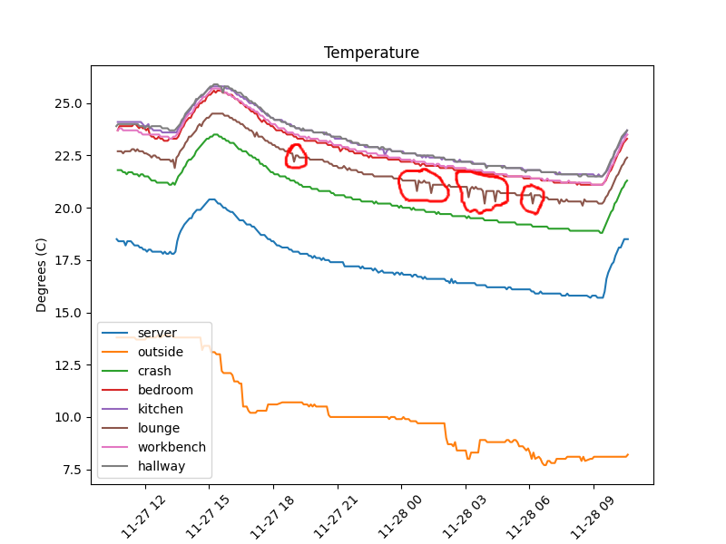
24-hour temperature graph of BME280 temperature data. Noise spikes highlighted in red.

The system samples the temperature from a BME280 environment sensor¹ every second (fs = 1Hz) and transmits the latest value at 5 minute intervals to a server which stores the data. The sensor was already configured to use oversampling as well as the inbuilt IIR filter yet the noise ‘spikes’ prevailed on this one board (labelled lounge in the figure). If the last measurement before the 5 minute interval was a noise fluctuation this would get transmitted to the server and manifest as a ‘spike’ as shown in the graph. In order to address this I decided to run the measurements through a single pole low pass filter in order to further ‘clean’ the noise spikes from the data.

What is it

The single pole low pass filter is a first-order IIR filter that replicates an analogue RC low pass filter in the digital realm². Some literature also refers to it as an exponentially weighted moving average filter ³. It requires two coefficients a0 and b1 which are the feed-forward (zero) and feed-backward (pole) components respectively^3,4. When used in the difference equation it takes the form:

y[n] = (x[n] * a0) + (y[n-1] * b1);

a0 is multiplied by the latest measurement x[n] and b1 is multiplied by the previous output of the filter y[n-1]. The coefficients are calculated by the following²:

a0 = 1 - alpha
b1 = alpha

where the alpha value is calculated by²:

alpha = e ^ (-2 * pi * fc/fs)

Here fc is the cut off frequency and fs is the sampling frequency, thus this value must lie in the range 0 < fc/fs < 0.5². Further algebra can simplify the difference equation as follows:

1.
y[n] = (x[n] * a0) + (y[n-1] * b1);

2.
y[n] = ((1 - alpha) * x[n] ) + (alpha * y[n-1])

3.
y[n] = (x[n] - (alpha * x[n]) ) + (alpha * y[n-1])

4.
y[n] = x[n] + (alpha * (y[n-1] - x[n]))

Python Modelling

For my use case I first modelled the filter using python so that I could inspect the step response⁵. My environment sensor is sampled every second, so the sampling rate fs would be 1Hz. In order to smooth random noise fluctuations / spikes I set the cutoff frequency fc to be 0.05Hz.

fs = 1
fc = 0.05
alpha = np.exp( -2 * np.pi * ( fc / fs ) )

This results in an alpha of 0.7304026910486456. This is then used in the difference equation to calculate the step response:

sig_len = 60 # a minute's worth of samples @ 1Hz
step = np.zeros(sig_len)
step[10:] = 1;

y = np.zeros(sig_len)
for i in range(0,sig_len):
    y[i] = step[i] + (alpha * (y[i-1] - step[i]))

The end result is shown in the plot below alongside the original step response. You can see that when the input signal changes from 0 to 1 it takes roughly 20 seconds (0.05Hz) to settle to the new value.

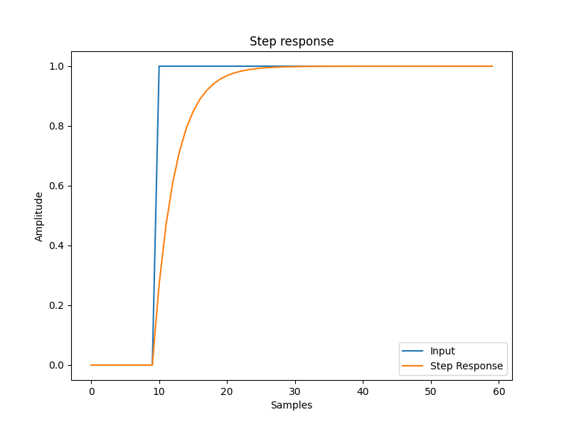
Step response of single pole LPF. fc=0.05Hz, fs=1Hz

Implementation

After modelling the step response I implemented the difference equation in C so that it could be used on an embedded target. The sensor data is stored and manipulated as a 64-bit floating point type double⁶ so it could be implemented as-is without any consideration for fixed point arithmetic:

#include <assert.h>

typedef struct
{
    double alpha;
    double y;
}
lpf_t;

extern void LPF_Init(lpf_t * filter)
{
    assert(filter != NULL);
    assert(filter->alpha > 0.0);
    assert(filter->alpha < 1.0);

    /* Initialise previous output of y as 0.0 */
    filter->y = 0.0;
}

extern double LPF_NextSample(lpf_t * filter, double x)
{
    assert(filter != NULL);
    /* y[n]   = x[n] + (alpha   * ( y[n-1] - x[n])) */
    filter->y = x + (filter->alpha * (filter->y - x));

    /* Return next output of filter */
    return filter->y;
}

These functions can then be used on incoming temperature data in order to filter out noise spikes:

double temperature_raw = BME280_ReadTemperature();
double filtered_temperature = LPF_NextSample(&filter, temperature_raw);

The end result is some nice graphs without noise fluctuations present as seen below⁷:

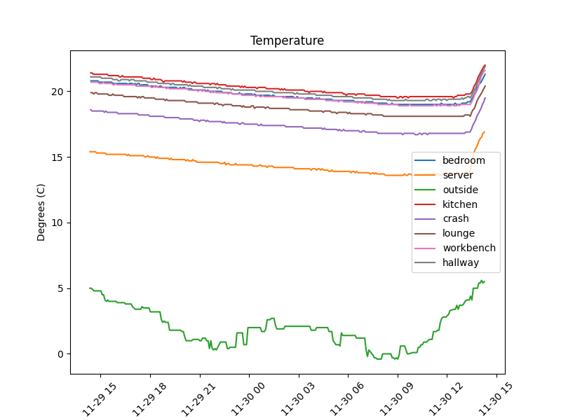
24-hour temperature graph of filtered BME280 temperature data.

Conclusion

It is always worth considering a low pass filter on your measurement data to remove noise fluctuations.

References

1. Bosch - Humidity sensor BME280 link ↩

2. The Scientist and Engineer’s Guide to Digital Signal Processing, Steven W. Smith, Second Edition, California Technical Publishing. link ↩ ↩² ↩³ ↩⁴

3. Wikipedia - Moving Average link ↩ ↩²

4. Foundations of Digital Signal Processing: Theory, algorithms and hardware design - Professor Patrick Gaydecki. link ↩

5. Wikipedia - Step Response link ↩

6. I am aware that reading and managing sensor data in a floating point type (especially a 64-bit one) on an embedded target is woefully inefficient but for this use case it is fine as there are very relaxed timing requirements. ↩

7. Note: the outside measurement comes from an external API, so that is used as-is with no filtering which is why it doesn’t look as “smooth” as the other measurements. ↩